Tutorial on the “Model Plot”
The hddm.plotting._plot_func_model model, which we can supply to
hddm.plotting.plot_from_data or hddm.plotting.plot_posteriors
functions has become quite versatile (complex).
This tutorial is meant to illustrate some of it’s capabilities. We can generate didactically useful plots of a variety of generative models. The LAN Tutorial also shows some of the usecases.
Install (colab)
# package to help train networks
# !pip install git+https://github.com/AlexanderFengler/LANfactory

# package containing simulators for ssms
# !pip install git+https://github.com/AlexanderFengler/ssm_simulators

# packages related to hddm
# !pip install cython
# !pip install pymc==2.3.8
# !pip install git+https://github.com/hddm-devs/kabuki
# !pip install git+https://github.com/hddm-devs/hddm
Import modules
# MODULE IMPORTS ----

# warning settings
import warnings

warnings.simplefilter(action="ignore", category=FutureWarning)

# Data management
import pandas as pd
import numpy as np
import pickle

# Plotting
import matplotlib.pyplot as plt
import matplotlib
import seaborn as sns

# Stats functionality
from statsmodels.distributions.empirical_distribution import ECDF

# HDDM
import hddm
from hddm.simulators.hddm_dataset_generators import simulator_h_c
Note a slight difference in how we treat generative models. Thanks to the LAN-extension, we have many generative models available to us, which we can broadbly classify as:
Legacy models, now titled:
ddm_hddm_baseandfull_ddm_hddm_base. Thefull_ddm_hddm_basemodel is used when any of thesv,storszparameters are positive.2-choice models enabled by the LAN-extension: amongst others the
levy,weibullandanglemodels.n-choice models enables by the LAN-extension: amongst others the
race_3andrace_4models.
The model plots work best with the 2-choice models enabled by the
LAN-extension. A n-choice version for the model plots exists (see
the _plot_func_model_n function) but is less well tested. Model
plots also work for the hddm_base models, however the positioning
of the reaction time and choice histograms is a little more tricky,
and will sometimes lead to unsatisfactory results.
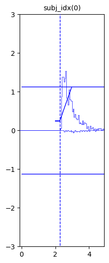
Example 1: Simple Data from ddm_hddm_base model
from hddm.simulators.hddm_dataset_generators import simulator_h_c
model = 'ddm_hddm_base'
n_samples = 1000

data, full_parameter_dict = simulator_h_c(
    n_subjects=1,
    n_trials_per_subject=n_samples,
    model=model,
    p_outlier=0.00,
    conditions=None,
    depends_on=None,
    regression_models=None,
    regression_covariates=None,
    group_only_regressors=False,
    group_only=None,
    fixed_at_default=None,
)
data
| rt | response | subj_idx | v | a | z | t | |
|---|---|---|---|---|---|---|---|
| 0 | 3.279359 | 1.0 | 0 | 1.241863 | 2.258145 | 0.605863 | 2.262367 |
| 1 | 2.632366 | 1.0 | 0 | 1.241863 | 2.258145 | 0.605863 | 2.262367 |
| 2 | 3.041361 | 1.0 | 0 | 1.241863 | 2.258145 | 0.605863 | 2.262367 |
| 3 | 2.648366 | 1.0 | 0 | 1.241863 | 2.258145 | 0.605863 | 2.262367 |
| 4 | 2.437368 | 1.0 | 0 | 1.241863 | 2.258145 | 0.605863 | 2.262367 |
| ... | ... | ... | ... | ... | ... | ... | ... |
| 995 | 2.478368 | 1.0 | 0 | 1.241863 | 2.258145 | 0.605863 | 2.262367 |
| 996 | 2.711365 | 1.0 | 0 | 1.241863 | 2.258145 | 0.605863 | 2.262367 |
| 997 | 3.343362 | 1.0 | 0 | 1.241863 | 2.258145 | 0.605863 | 2.262367 |
| 998 | 2.670366 | 1.0 | 0 | 1.241863 | 2.258145 | 0.605863 | 2.262367 |
| 999 | 2.893363 | 1.0 | 0 | 1.241863 | 2.258145 | 0.605863 | 2.262367 |
1000 rows × 7 columns
hddm.plotting.plot_from_data(df = data,
                            generative_model = model,
                            save = False,
                            make_transparent = False,
                            path = 'tmp_figures',
                            value_range = np.arange(-.1, 5, 0.1),
                            plot_func = hddm.plotting._plot_func_model,
                            keep_frame = True,
                            **{'hist_bottom': 0.})
plt.show()
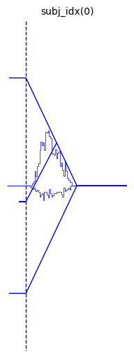
Example 2: Simple Data from a model enabled by LAN-extension
from hddm.simulators.hddm_dataset_generators import simulator_h_c
model = 'angle'
n_samples = 1000

data, full_parameter_dict = simulator_h_c(
    n_subjects=1,
    n_trials_per_subject=n_samples,
    model=model,
    p_outlier=0.00,
    conditions=None,
    depends_on=None,
    regression_models=None,
    regression_covariates=None,
    group_only_regressors=False,
    group_only=None,
    fixed_at_default=None,
)
data
| rt | response | subj_idx | v | a | z | t | theta | |
|---|---|---|---|---|---|---|---|---|
| 0 | 1.117624 | 1.0 | 0 | 0.832015 | 1.953756 | 0.426032 | 0.685626 | 0.745569 |
| 1 | 2.047633 | 0.0 | 0 | 0.832015 | 1.953756 | 0.426032 | 0.685626 | 0.745569 |
| 2 | 1.491619 | 1.0 | 0 | 0.832015 | 1.953756 | 0.426032 | 0.685626 | 0.745569 |
| 3 | 1.583618 | 1.0 | 0 | 0.832015 | 1.953756 | 0.426032 | 0.685626 | 0.745569 |
| 4 | 1.662617 | 1.0 | 0 | 0.832015 | 1.953756 | 0.426032 | 0.685626 | 0.745569 |
| ... | ... | ... | ... | ... | ... | ... | ... | ... |
| 995 | 1.283622 | 0.0 | 0 | 0.832015 | 1.953756 | 0.426032 | 0.685626 | 0.745569 |
| 996 | 2.259643 | 1.0 | 0 | 0.832015 | 1.953756 | 0.426032 | 0.685626 | 0.745569 |
| 997 | 1.866625 | 0.0 | 0 | 0.832015 | 1.953756 | 0.426032 | 0.685626 | 0.745569 |
| 998 | 1.129624 | 1.0 | 0 | 0.832015 | 1.953756 | 0.426032 | 0.685626 | 0.745569 |
| 999 | 2.129637 | 1.0 | 0 | 0.832015 | 1.953756 | 0.426032 | 0.685626 | 0.745569 |
1000 rows × 8 columns
hddm.plotting.plot_from_data(df = data,
                            generative_model = model,
                            save = False,
                            make_transparent = False,
                            path = 'tmp_figures',
                            value_range = np.arange(-.1, 5, 0.1),
                            plot_func = hddm.plotting._plot_func_model,
                            keep_frame = False,
                            **{'hist_bottom': 0})
plt.show()
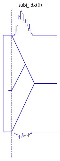
We can move around the histograms with the hist_bottom, argument
(kwarg).
hddm.plotting.plot_from_data(df = data,
                            generative_model = model,
                            save = False,
                            make_transparent = False,
                            path = 'tmp_figures',
                            value_range = np.arange(-.1, 5, 0.1),
                            plot_func = hddm.plotting._plot_func_model,
                            keep_frame = False,
                            **{'hist_bottom': data.a.values[0],
                               'ylim': 3})
plt.show()
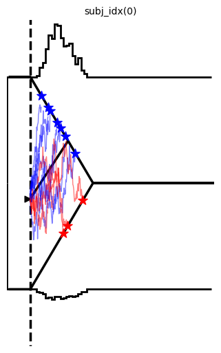
We can look at a few other arguments to illustrate the range of styling options.
hddm.plotting.plot_from_data(df = data,
                            generative_model = model,
                            save = False,
                            make_transparent = False,
                            path = 'tmp_figures',
                            value_range = np.arange(-.1, 7, 0.1),
                            plot_func = hddm.plotting._plot_func_model,
                            keep_frame = False,
                            figsize = (14, 6),
                            **{"hist_bottom": data.a.values[0],
                               "ylim": 3,
                                "add_trajectories": True,
                                "n_trajectories": 10,
                                "markersize_trajectory_rt_choice": 100,
                                "markertype_trajectory_rt_choice": "*",
                                "color_trajectories": {-1.:"red", 1.:"blue"},
                                "markercolor_trajectory_rt_choice": {-1.:"red",1.:'blue'},
                                "add_data_model_markersize_starting_point": 40,
                                "add_data_model_markertype_starting_point": '>',
                                "add_data_model_markershift_starting_point": -0.1,
                                "linewidth_histogram": 2,
                                "linewidth_model": 2,
                                "bin_size": 0.1,
                                "data_color": "black"})
plt.show()
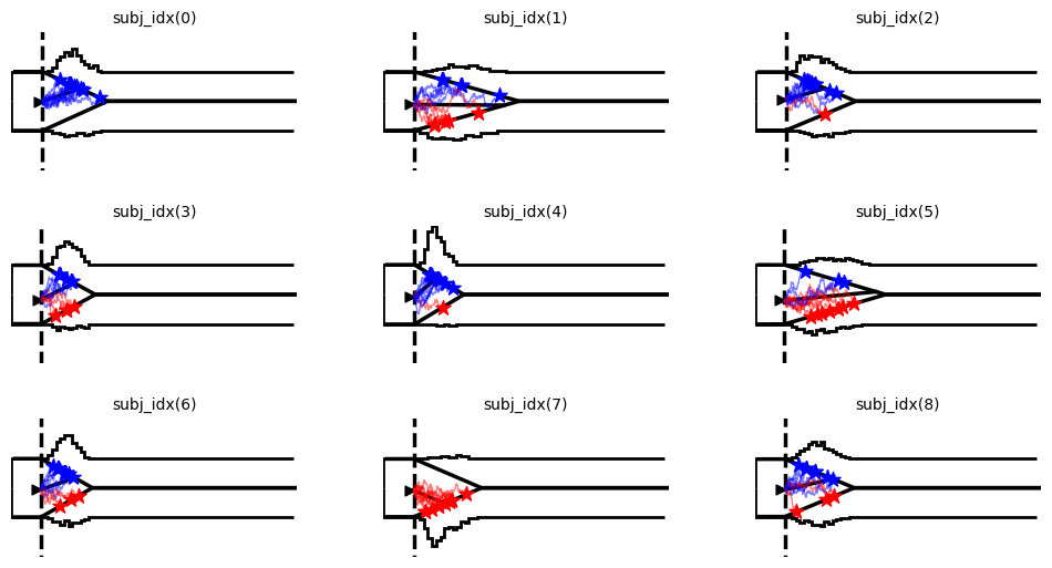
Example 3: More complex data
model = 'angle'
n_samples = 500

data, full_parameter_dict = simulator_h_c(
    n_subjects=9,
    n_trials_per_subject=n_samples,
    model=model,
    p_outlier=0.00,
    conditions=None,
    depends_on=None,
    regression_models=None,
    regression_covariates=None,
    group_only_regressors=False,
    group_only=None,
    fixed_at_default=None,
)
hddm.plotting.plot_from_data(df = data,
                            generative_model = model,
                            save = False,
                            columns = 3,
                            make_transparent = False,
                            path = 'tmp_figures',
                            value_range = np.arange(-.1, 7, 0.1),
                            plot_func = hddm.plotting._plot_func_model,
                            keep_frame = False,
                            figsize = (12, 6),
                            **{"hist_bottom": data.a.values[0],
                               "ylim": 4,
                                "add_trajectories": True,
                                "n_trajectories": 10,
                                "markersize_trajectory_rt_choice": 100,
                                "markertype_trajectory_rt_choice": "*",
                                "color_trajectories": {-1.:"red", 1.:"blue"},
                                "markercolor_trajectory_rt_choice": {-1.:"red",1.:'blue'},
                                "add_data_model_markersize_starting_point": 40,
                                "add_data_model_markertype_starting_point": '>',
                                "add_data_model_markershift_starting_point": -0.1,
                                "linewidth_histogram": 2,
                                "linewidth_model": 2,
                                "bin_size": 0.1,
                                "data_color": "black"})
plt.show()
Example 4: Making gifs
Using the model plot, we can create fairly exciting gifs to illustrate the workings of various Sequential Sampling Models.
import os
import imageio # package for gifs
from hddm.simulators.basic_simulator import simulator
from hddm.simulators import hddm_preprocess


#
theta = np.array([[.1, .6, 0.5, .5]])
theta_secondary = np.array([-.3, 1., 0.5, 1.0])
model = 'ddm'
model_secondary = 'ddm'
n_samples=20000
n_samples_secondary=500 # If we want to have another reference dataset (can be useful for illustrating e.g. likelihood)

create_frames=True
make_gif=True
add_secondary_data=False

# Create trajectories (have to presimulate, then use for frame generation)
n_trajectories = 1
trajectories = []
trajectory_choices = []
for i in range(n_trajectories):
    out_tmp = hddm.simulators.basic_simulator.simulator(theta = theta,
                                                        model = model,
                                                        n_samples = 1,
                                                        delta_t = 0.001)
    trajectories.append(out_tmp[2]['trajectory'].T)
    trajectory_choices.append(out_tmp[1].flatten())

trajectories_to_supply = np.concatenate(trajectories)
trajectory_choices_to_supply = np.concatenate(trajectory_choices)

trajectory_supply_dict = {'trajectories': trajectories_to_supply,
                          'trajectory_choices':trajectory_choices_to_supply}

# Create data
out = simulator(theta = theta,
                model = model,
                n_samples = n_samples,
                delta_t = 0.001)

data = hddm_preprocess(out,
                       subj_id = '0',
                       add_model_parameters = True)

out_secondary = simulator(theta = theta_secondary,
                          model = model_secondary,
                          n_samples = n_samples_secondary,
                          delta_t = 0.001)

data_secondary = hddm_preprocess(out_secondary,
                       subj_id = '0',
                       add_model_parameters = True)


if create_frames:
    frames = []
    cnt = 0
    for i in range(n_trajectories):
        # Subset precomputed trajectories for current plot
        tmp_trajectories = {}
        tmp_trajectories['trajectories'] = trajectory_supply_dict['trajectories'][:(i + 1), :]
        tmp_trajectories['trajectory_choices'] = trajectory_supply_dict['trajectory_choices'][:(i + 1)]
        tmp_maxid = np.argmax(np.where(tmp_trajectories['trajectories'][i, :] > -999))

        for j in range(10, tmp_maxid + 110, 10):
            # Define all the plot options via a kwarg dict
            plot_options_dict = {"alpha": 1.0, "ylim": 3.0,
                                "hist_bottom": data.a.values[0],
                                "add_data_rts": True, "add_data_model": True,
                                'add_trajectories': True,
                                "alpha_trajectories": 0.1,
                                'n_trajectories': None,
                                "supplied_trajectory": tmp_trajectories, #out[2]['trajectory'][:, 0][np.arange(0, out[2]['trajectory'][:, 0].shape[0], 10)],
                                "maxid_supplied_trajectory": j,
                                "color_trajectories": {-1.:"red", 1.:"blue"},
                                "data_color": "black",
                                "bin_size": 0.1,
                                "linewidth_histogram": 2,
                                "linewidth_model": 2,
                                "markersize_trajectory_rt_choice": 100,
                                "markertype_trajectory_rt_choice": "*",
                                "markercolor_trajectory_rt_choice": {-1.:"red",1.:'blue'},
                                "highlight_trajectory_rt_choice": True,
                                "add_data_model_keep_boundary": True,
                                "add_data_model_keep_slope": True,
                                "add_data_model_keep_ndt": True,
                                "add_data_model_keep_starting_point": True,
                                "add_data_model_markersize_starting_point": 40,
                                "add_data_model_markertype_starting_point": '>',
                                "add_data_model_markershift_starting_point": -0.05,
                                "secondary_data": None, #data_secondary,
                                "secondary_data_color": 'blue',
                                "secondary_data_label": None}

            # Create plot
            hddm.plotting.plot_from_data(
                                        df=data,
                                        generative_model=model,
                                        save=True,
                                        make_transparent = False,
                                        path='tmp_figures',
                                        save_name='myfig_' + str(cnt),
                                        columns=1,
                                        groupby=["subj_idx"],
                                        figsize=(6, 4),
                                        value_range=np.arange(-.2, 5, 0.1),
                                        delta_t_model = 0.001,
                                        keep_frame=False,
                                        keep_title=False,
                                        plot_func=hddm.plotting._plot_func_model,
                                        **plot_options_dict)

            plt.close('all')

            # Read image, append to frames and delete it from disk
            image = imageio.v2.imread('./tmp_figures/myfig_' + str(cnt) + '.png')
            frames.append(image)
            os.remove('./tmp_figures/myfig_' + str(cnt) + '.png')

            cnt += 1
    # Append a few frames with the last image to make the gif a bit better to view
    for j in range(100):
        frames.append(image)

imageio.mimsave('./tmp_gifs/example.gif',
                frames,
                fps = 50)
SegmentLocal