Posterior Predictive Checks

In this tutorial you will learn how to run posterior predictive checks in HDDM.

A posterior predictive check is a very useful tool when you want to evaluate if your model can reproduce key patterns in your data. Specifically, you can define a summary statistic that describes the pattern you are interested in (e.g. accuracy in your task) and then simulate new data from the posterior of your fitted model. You can the apply the the summary statistic to each of the data sets you simulated from the posterior and see if the model does a good job of reproducing this pattern by comparing the summary statistics from the simulations to the summary statistic caluclated over the model.

What is critical is that you do not only get a single summary statistic from the simulations but a whole distribution which captures the uncertainty in our model estimate.

Lets do a simple analysis using simulated data. First, import HDDM.

import hddm

Simulate data from known parameters and two conditions (easy and hard).

data, params = hddm.generate.gen_rand_data(params={'easy': {'v': 1, 'a': 2, 't': .3},
                                                   'hard': {'v': 1, 'a': 2, 't': .3}})

First, lets estimate the same model that was used to generate the data.

m = hddm.HDDM(data, depends_on={'v': 'condition'})
m.sample(1000, burn=20)

Next, we’ll want to simulate data from the model. By default, post_pred_gen() will use 500 parameter values from the posterior (i.e. posterior samples) and simulate a different data set for each parameter value.

ppc_data = hddm.utils.post_pred_gen(m)

The returned data structure is a pandas DataFrame object with a hierarchical index.

ppc_data.head(10)

			rt	response
node	sample
wfpt(easy)	0	0	0.41009	1
		1	0.79089	1
		2	-0.67769	0
		3	0.49359	1
		4	1.59039	1
		5	0.99669	1
		6	5.51089	1
		7	0.73069	1
		8	0.82829	1
		9	0.92839	1

The first level of the DataFrame contains each observed node. In this case the easy condition. If we had multiple subjects we would get one for each subject.

The second level contains the simulated data sets. Since we simulated 500, these will go from 0 to 499 – each with generated from a different parameter value sampled from the posterior.

The third level is the same index as used in the data and numbers each trial in your data.

For more information on how to work with hierarchical indices, see the Pandas documentation.

There are also some helpful options like append_data you can pass to post_pred_gen().

help(hddm.utils.post_pred_gen)

Help on function post_pred_gen in module kabuki.analyze:

post_pred_gen(model, groupby=None, samples=500, append_data=False, progress_bar=True)
    Run posterior predictive check on a model.

    :Arguments:
        model : kabuki.Hierarchical
            Kabuki model over which to compute the ppc on.

    :Optional:
        samples : int
            How many samples to generate for each node.
        groupby : list
            Alternative grouping of the data. If not supplied, uses splitting
            of the model (as provided by depends_on).
        append_data : bool (default=False)
            Whether to append the observed data of each node to the replicatons.
        progress_bar : bool (default=True)
            Display progress bar

    :Returns:
        Hierarchical pandas.DataFrame with multiple sampled RT data sets.
        1st level: wfpt node
        2nd level: posterior predictive sample
        3rd level: original data index

    :See also:
        post_pred_stats

Now we want to compute the summary statistics over each simulated data set and compare that to the summary statistic of our actual data by calling post_pred_stats().

ppc_compare = hddm.utils.post_pred_stats(data, ppc_data)

print ppc_compare

          observed      mean       std       SEM       MSE  credible  \

stat
accuracy  0.890000  0.874580  0.063930  0.000238  0.004325         1
mean_ub   1.084831  1.048314  0.111169  0.001334  0.013692         1
std_ub    0.654891  0.542704  0.129186  0.012586  0.029275         1
10q_ub    0.510200  0.549030  0.045206  0.001508  0.003551         1
30q_ub    0.649200  0.704437  0.067714  0.003051  0.007636         1
50q_ub    0.818000  0.891622  0.099117  0.005420  0.015244         1
70q_ub    1.253800  1.165027  0.149496  0.007881  0.030230         1
90q_ub    1.884400  1.741424  0.282329  0.020442  0.100152         1
mean_lb  -0.970818 -1.046499  0.269939  0.005728  0.078595         1
std_lb    0.543502  0.423627  0.251797  0.014370  0.077772         1
10q_lb    0.547000  0.660271  0.203289  0.012830  0.054157         1
30q_lb    0.648000  0.785022  0.223779  0.018775  0.068852         1
50q_lb    0.693000  0.939898  0.269239  0.060958  0.133448         1
70q_lb    1.022000  1.158692  0.346341  0.018685  0.138637         1
90q_lb    1.666000  1.532752  0.515372  0.017755  0.283363         1

           quantile  mahalanobis
stat
accuracy  55.500000     0.241202
mean_ub   64.699997     0.328490
std_ub    81.500000     0.868420
10q_ub    18.900000     0.858949
30q_ub    20.700001     0.815736
50q_ub    23.400000     0.742775
70q_ub    73.500000     0.593812
90q_ub    71.500000     0.506417
mean_lb   57.517658     0.280362
std_lb    72.754791     0.476077
10q_lb    26.538849     0.557192
30q_lb    25.933401     0.612307
50q_lb    14.228052     0.917022
70q_lb    40.060543     0.394675
90q_lb    65.893036     0.258547

As you can see, we did not have to define the summary statistics as by default, HDDM already calculates a bunch of useful statistics for RT analysis such as the accuracy, mean RT of the upper and lower boundary (ub and lb respectively), standard deviation and quantiles. These are listed in the rows of the DataFrame.

For each distribution of summary statistics there are multiple ways to compare them to the summary statistic obtained on the observerd data. These are listed in the columns. observed is just the value of the summary statistic of your data. mean is the mean of the summary statistics of the simulated data sets (they should be a good match if the model reproduces them). std is a measure of how much variation is produced in the summary statistic.

The rest of the columns are measures of how far the summary statistic of the data is away from the summary statistics of the simulated data. SEM = standard error from the mean, MSE = mean-squared error, credible = in the 95% credible interval.

Finally, we can also tell post_pred_stats() to return the summary statistics themselves by setting call_compare=False:

ppc_stats = hddm.utils.post_pred_stats(data, ppc_data, call_compare=False)

print ppc_stats.head()

                 accuracy   mean_ub    std_ub    10q_ub    30q_ub    50q_ub  \

(wfpt(easy), 0)      0.96  1.164858  0.825420  0.500940  0.736800  0.909940
(wfpt(easy), 1)      0.92  1.066229  0.500696  0.552553  0.725853  0.842753
(wfpt(easy), 2)      0.84  1.106792  0.660981  0.538767  0.708527  0.852747
(wfpt(easy), 3)      0.90  0.949962  0.524693  0.507878  0.634398  0.784638
(wfpt(easy), 4)      0.88  0.967202  0.523246  0.509131  0.638661  0.781231

                   70q_ub    90q_ub   mean_lb    std_lb    10q_lb    30q_lb  \

(wfpt(easy), 0)  1.388660  1.902310 -1.270140  0.592450  0.796180  1.033160
(wfpt(easy), 1)  1.298903  1.815803 -0.921803  0.204067  0.720703  0.842803
(wfpt(easy), 2)  1.137547  1.791117 -1.610109  1.577114  0.813307  0.843867
(wfpt(easy), 3)  1.013418  1.533458 -1.125698  0.371009  0.667518  1.004518
(wfpt(easy), 4)  0.958081  1.826761 -0.765531  0.363230  0.545531  0.599181

                   50q_lb    70q_lb    90q_lb
(wfpt(easy), 0)  1.270140  1.507120  1.744100
(wfpt(easy), 1)  0.899403  0.964963  1.140823
(wfpt(easy), 2)  1.084597  1.183127  2.654677
(wfpt(easy), 3)  1.334438  1.347158  1.454438
(wfpt(easy), 4)  0.614681  0.665531  1.136381

This DataFrame has a row for each simulated data set. The columns are the different summary statistics.

Defining your own summary statistics

You can also define your own summary statistics and pass them to post_pred_stats():

ppc_stats = hddm.utils.post_pred_stats(data, ppc_data, stats=lambda x: np.mean(x), call_compare=False)

ppc_stats.head()

	stat
(wfpt(easy), 0)	1.067459
(wfpt(easy), 1)	0.907187
(wfpt(easy), 2)	0.672088
(wfpt(easy), 3)	0.742396
(wfpt(easy), 4)	0.759274

Note that stats can also be a dictionary mapping the name of the summary statistic to its function.

Using PPC for model comparison with the groupby argument

One useful application of PPC is to perform model comparison. Specifically, you might estimate two models, one for which a certain parameter is split for a condition (say drift-rate v for hard and easy conditions to stay with our example above) and one in which those conditions are pooled and you only estimate one drift-rate.

You then want to test which model explains the data better to assess whether the two conditions are really different. To do this, we can generate data from both models and see if the pooled model systematically misses aspects of the RT data of the two conditions. This is what the groupby keyword argument is for. Without it, if you ran post_pred_gen() on the pooled model you would get simulated RT data which was not split by conditions. Note that while the RT data will be split by condition, the exact same parameters are used to simulate data of the two conditions as the pooled model does not separate them. It simply allows us to match the two conditions present in the data to the jointly simulated data more easily.

m_pooled = hddm.HDDM(data) # v does not depend on conditions
m_pooled.sample(1000, burn=20)

ppc_data_pooled = hddm.utils.post_pred_gen(m_pooled, groupby=['condition'])

You could then compare ppc_data_pooled to ppc_data above (by passing them to post_pred_stats) and find that the model with separate drift-rates accounts for accuracy (mean_ub) in both conditions, while the pooled model can’t account for accuracy in either condition (e.g. lower MSE).

Summary statistics relating to outside variables

Another useful way to apply posterior predictive checks is if you have trial-by-trial measure (e.g. EEG brain measure). In that case the append_data keyword argument is useful.

Lets add a dummy column to our data. This is going to be uncorrelated to anything but you’ll get the idea.

from numpy.random import randn
data['trlbytrl'] = randn(len(data))

m_reg = hddm.HDDMRegressor(data, 'v ~ trlbytrl')
m_reg.sample(1000, burn=20)

ppc_data = hddm.utils.post_pred_gen(m_reg, append_data=True)

from scipy.stats import linregress
ppc_regression = []
for (node, sample), sim_data in ppc_data.groupby(level=(0, 1)):
    ppc_regression.append(linregress(sim_data.trlbytrl, sim_data.rt_sampled)[0]) # slope

orig_regression = linregress(data.trlbytrl, data.rt)[0]

plt.hist(ppc_regression)
plt.axvline(orig_regression, c='r', lw=3)
plt.xlabel('slope')

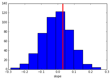
As you can see, the simulated data sets have on average no correlation to our trial-by-trial measure (just as in the data) but we also get a nice sense of the uncertainty in our estimation.