Posterior Predictive Checks
In this tutorial you will learn how to run posterior predictive checks in HDDM.
A posterior predictive check is a very useful tool when you want to evaluate if your model can reproduce key patterns in your data. Specifically, you can define a summary statistic that describes the pattern you are interested in (e.g. accuracy in your task) and then simulate new data from the posterior of your fitted model. You can the apply the the summary statistic to each of the data sets you simulated from the posterior and see if the model does a good job of reproducing this pattern by comparing the summary statistics from the simulations to the summary statistic caluclated over the model.
What is critical is that you do not only get a single summary statistic from the simulations but a whole distribution which captures the uncertainty in our model estimate.
Lets do a simple analysis using simulated data. First, import HDDM.
import hddm
import matplotlib.pyplot as plt
import numpy as np
%matplotlib inline

import warnings
warnings.filterwarnings('ignore')
Simulate data from known parameters and two conditions (easy and hard).
data, params = hddm.generate.gen_rand_data(params={'easy': {'v': 1, 'a': 2, 't': .3},
                                                   'hard': {'v': 1, 'a': 2, 't': .3}})
First, lets estimate the same model that was used to generate the data.
m = hddm.HDDM(data, depends_on={'v': 'condition'})
m.sample(1000, burn=20)
No model attribute --> setting up standard HDDM
Set model to ddm
 [-----------------100%-----------------] 1000 of 1000 complete in 12.5 sec
<pymc.MCMC.MCMC at 0x104066090>
Next, we’ll want to simulate data from the model. By default,
post_pred_gen() will use 500 parameter values from the posterior
(i.e. posterior samples) and simulate a different data set for each
parameter value.
print(m.nodes_db)
           knode_name stochastic observed   subj        node      tag  a                   a       True    False  False           a       ()
v(easy)             v       True    False  False     v(easy)  (easy,)
v(hard)             v       True    False  False     v(hard)  (hard,)
t                   t       True    False  False           t       ()
wfpt(easy)       wfpt      False     True  False  wfpt(easy)  (easy,)
wfpt(hard)       wfpt      False     True  False  wfpt(hard)  (hard,)

                depends hidden   rt response subj_idx condition      mean  a                    []  False  NaN      NaN      NaN       NaN   1.90643
v(easy)     [condition]  False  NaN      NaN      NaN      easy   1.06179
v(hard)     [condition]  False  NaN      NaN      NaN      hard  0.943137
t                    []  False  NaN      NaN      NaN       NaN  0.341715
wfpt(easy)  [condition]  False  NaN      NaN      NaN      easy       NaN
wfpt(hard)  [condition]  False  NaN      NaN      NaN      hard       NaN

                  std      2.5q       25q       50q       75q     97.5q  a            0.123325   1.70192   1.81497   1.89453   1.97966   2.18115
v(easy)      0.213885  0.672581  0.925245   1.05542    1.1914   1.49813
v(hard)       0.17852  0.605106  0.817572  0.944719   1.06105   1.27941
t           0.0261543  0.278789  0.325973  0.344599  0.362117  0.383125
wfpt(easy)        NaN       NaN       NaN       NaN       NaN       NaN
wfpt(hard)        NaN       NaN       NaN       NaN       NaN       NaN

                mc err
a           0.00666755
v(easy)     0.00718197
v(hard)     0.00616936
t           0.00127485
wfpt(easy)         NaN
wfpt(hard)         NaN
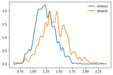
hddm.analyze.plot_posterior_nodes(m.nodes_db.loc[['v(easy)', 'v(hard)'], 'node'])
ppc_data = hddm.utils.post_pred_gen(m)
[--------------------------150%---------------------------] 3 of 2 complete in 5.9 sec
hddm.utils.post_pred_stats(data, ppc_data)
| observed | mean | std | SEM | MSE | credible | quantile | mahalanobis | |
|---|---|---|---|---|---|---|---|---|
| stat | ||||||||
| accuracy | 0.910000 | 0.927500 | 0.050637 | 0.000306 | 0.002870 | True | 31.500000 | 0.345593 |
| mean_ub | 0.935440 | 0.951484 | 0.098785 | 0.000257 | 0.010016 | True | 46.400002 | 0.162416 |
| std_ub | 0.421473 | 0.464852 | 0.111991 | 0.001882 | 0.014424 | True | 37.700001 | 0.387345 |
| 10q_ub | 0.501000 | 0.521309 | 0.039991 | 0.000412 | 0.002012 | True | 32.200001 | 0.507850 |
| 30q_ub | 0.686000 | 0.658764 | 0.057687 | 0.000742 | 0.004070 | True | 71.500000 | 0.472135 |
| 50q_ub | 0.832000 | 0.820630 | 0.088531 | 0.000129 | 0.007967 | True | 59.900002 | 0.128429 |
| 70q_ub | 1.008000 | 1.053636 | 0.134238 | 0.002083 | 0.020102 | True | 40.200001 | 0.339962 |
| 90q_ub | 1.573000 | 1.542863 | 0.247801 | 0.000908 | 0.062314 | True | 59.599998 | 0.121618 |
| mean_lb | -1.049667 | -0.990737 | 0.350941 | 0.003473 | 0.126632 | True | 33.798283 | 0.167918 |
| std_lb | 0.430255 | 0.297619 | 0.251784 | 0.017592 | 0.080988 | True | 74.248924 | 0.526784 |
| 10q_lb | 0.491400 | 0.726807 | 0.332695 | 0.055416 | 0.166103 | True | 9.442060 | 0.707575 |
| 30q_lb | 0.799600 | 0.819943 | 0.335312 | 0.000414 | 0.112848 | True | 61.266094 | 0.060669 |
| 50q_lb | 1.130000 | 0.928716 | 0.356847 | 0.040515 | 0.167855 | True | 80.686699 | 0.564064 |
| 70q_lb | 1.192800 | 1.076653 | 0.398996 | 0.013490 | 0.172688 | True | 69.849785 | 0.291099 |
| 90q_lb | 1.516800 | 1.302383 | 0.520954 | 0.045975 | 0.317368 | True | 71.995705 | 0.411585 |
The returned data structure is a pandas DataFrame object with a
hierarchical index.
ppc_data.head(10)
| rt | response | |||
|---|---|---|---|---|
| node | sample | |||
| wfpt(easy) | 0 | 0 | 0.481109 | 1 |
| 1 | 0.755106 | 1 | ||
| 2 | 0.713106 | 1 | ||
| 3 | 1.100101 | 1 | ||
| 4 | 0.905104 | 1 | ||
| 5 | 0.716106 | 1 | ||
| 6 | -0.873104 | 0 | ||
| 7 | 0.404109 | 1 | ||
| 8 | 1.566114 | 1 | ||
| 9 | 1.419107 | 1 |
The first level of the DataFrame contains each observed node. In
this case the easy condition. If we had multiple subjects we would get
one for each subject.
The second level contains the simulated data sets. Since we simulated 500, these will go from 0 to 499 – each with generated from a different parameter value sampled from the posterior.
The third level is the same index as used in the data and numbers each trial in your data.
For more information on how to work with hierarchical indices, see the Pandas documentation.
There are also some helpful options like append_data you can pass to
post_pred_gen().
help(hddm.utils.post_pred_gen)
Help on function post_pred_gen in module kabuki.analyze:

post_pred_gen(model, groupby=None, samples=500, append_data=False, add_model_parameters=False, progress_bar=True)
    Run posterior predictive check on a model.

    :Arguments:
        model : kabuki.Hierarchical
            Kabuki model over which to compute the ppc on.

    :Optional:
        samples : int
            How many samples to generate for each node.
        groupby : list
            Alternative grouping of the data. If not supplied, uses splitting
            of the model (as provided by depends_on).
        append_data : bool (default=False)
            Whether to append the observed data of each node to the replicatons.
        progress_bar : bool (default=True)
            Display progress bar

    :Returns:
        Hierarchical pandas.DataFrame with multiple sampled RT data sets.
        1st level: wfpt node
        2nd level: posterior predictive sample
        3rd level: original data index

    :See also:
        post_pred_stats
Now we want to compute the summary statistics over each simulated data
set and compare that to the summary statistic of our actual data by
calling post_pred_stats().
ppc_compare = hddm.utils.post_pred_stats(data, ppc_data)
print(ppc_compare)
          observed      mean       std       SEM       MSE credible  stat
accuracy  0.910000  0.927500  0.050637  0.000306  0.002870     True
mean_ub   0.935440  0.951484  0.098785  0.000257  0.010016     True
std_ub    0.421473  0.464852  0.111991  0.001882  0.014424     True
10q_ub    0.501000  0.521309  0.039991  0.000412  0.002012     True
30q_ub    0.686000  0.658764  0.057687  0.000742  0.004070     True
50q_ub    0.832000  0.820630  0.088531  0.000129  0.007967     True
70q_ub    1.008000  1.053636  0.134238  0.002083  0.020102     True
90q_ub    1.573000  1.542863  0.247801  0.000908  0.062314     True
mean_lb  -1.049667 -0.990737  0.350941  0.003473  0.126632     True
std_lb    0.430255  0.297619  0.251784  0.017592  0.080988     True
10q_lb    0.491400  0.726807  0.332695  0.055416  0.166103     True
30q_lb    0.799600  0.819943  0.335312  0.000414  0.112848     True
50q_lb    1.130000  0.928716  0.356847  0.040515  0.167855     True
70q_lb    1.192800  1.076653  0.398996  0.013490  0.172688     True
90q_lb    1.516800  1.302383  0.520954  0.045975  0.317368     True

           quantile  mahalanobis
stat
accuracy  31.500000     0.345593
mean_ub   46.400002     0.162416
std_ub    37.700001     0.387345
10q_ub    32.200001     0.507850
30q_ub    71.500000     0.472135
50q_ub    59.900002     0.128429
70q_ub    40.200001     0.339962
90q_ub    59.599998     0.121618
mean_lb   33.798283     0.167918
std_lb    74.248924     0.526784
10q_lb     9.442060     0.707575
30q_lb    61.266094     0.060669
50q_lb    80.686699     0.564064
70q_lb    69.849785     0.291099
90q_lb    71.995705     0.411585
As you can see, we did not have to define the summary statistics as by
default, HDDM already calculates a bunch of useful statistics for RT
analysis such as the accuracy, mean RT of the upper and lower boundary
(ub and lb respectively), standard deviation and quantiles. These are
listed in the rows of the DataFrame.
For each distribution of summary statistics there are multiple ways to
compare them to the summary statistic obtained on the observerd data.
These are listed in the columns. observed is just the value of the
summary statistic of your data. mean is the mean of the summary
statistics of the simulated data sets (they should be a good match if
the model reproduces them). std is a measure of how much variation
is produced in the summary statistic.
The rest of the columns are measures of how far the summary statistic of
the data is away from the summary statistics of the simulated data.
SEM = standard error from the mean, MSE = mean-squared error,
credible = in the 95% credible interval.
Finally, we can also tell post_pred_stats() to return the summary
statistics themselves by setting call_compare=False:
ppc_stats = hddm.utils.post_pred_stats(data, ppc_data, call_compare=False)
print(ppc_stats.head())
                   accuracy   mean_ub    std_ub    10q_ub    30q_ub    50q_ub  node       sample
wfpt(easy) 0           0.86  1.062849  0.724248  0.484509  0.667707  0.905104
           1           0.98  0.977835  0.474633  0.498661  0.680059  0.882057
           2           0.82  0.996223  0.515579  0.555150  0.671149  0.817147
           3           0.88  0.875679  0.305067  0.510363  0.733061  0.835860
           4           0.92  0.815038  0.503699  0.510257  0.593757  0.626257

                     70q_ub    90q_ub   mean_lb    std_lb    10q_lb    30q_lb  node       sample
wfpt(easy) 0       1.078501  1.749323 -1.398971  0.610027  0.740706  1.084301
           1       1.133453  1.642467 -0.624060  0.000000  0.624060  0.624060
           2       1.004145  1.785162 -1.002371  0.407241  0.611750  0.756748
           3       0.951658  1.376258 -0.928192  0.198288  0.706861  0.757861
           4       0.779755  1.143250 -1.067014  0.635796  0.646857  0.666057

                     50q_lb    70q_lb    90q_lb
node       sample
wfpt(easy) 0       1.268101  1.595516  2.214336
           1       0.624060  0.624060  0.624060
           2       0.802147  1.145143  1.375747
           3       0.916359  1.091857  1.161356
           4       0.733756  0.934758  1.753776
This DataFrame has a row for each simulated data set. The columns
are the different summary statistics.
Using PPC for model comparison with the groupby argument
One useful application of PPC is to perform model comparison.
Specifically, you might estimate two models, one for which a certain
parameter is split for a condition (say drift-rate v for hard and
easy conditions to stay with our example above) and one in which those
conditions are pooled and you only estimate one drift-rate.
You then want to test which model explains the data better to assess
whether the two conditions are really different. To do this, we can
generate data from both models and see if the pooled model
systematically misses aspects of the RT data of the two conditions. This
is what the groupby keyword argument is for. Without it, if you ran
post_pred_gen() on the pooled model you would get simulated RT data
which was not split by conditions. Note that while the RT data will be
split by condition, the exact same parameters are used to simulate data
of the two conditions as the pooled model does not separate them. It
simply allows us to match the two conditions present in the data to the
jointly simulated data more easily.
m_pooled = hddm.HDDM(data) # v does not depend on conditions
m_pooled.sample(1000, burn=20)
ppc_data_pooled = hddm.utils.post_pred_gen(m_pooled, groupby=['condition'])
You could then compare ppc_data_pooled to ppc_data above (by
passing them to post_pred_stats) and find that the model with
separate drift-rates accounts for accuracy (mean_ub) in both
conditions, while the pooled model can’t account for accuracy in either
condition (e.g. lower MSE).
Defining your own summary statistics
You can also define your own summary statistics and pass them to
post_pred_stats():
ppc_stats = hddm.utils.post_pred_stats(data, ppc_data, stats=lambda x: np.mean(x), call_compare=False)
ppc_stats.head()
| stat | ||
|---|---|---|
| node | sample | |
| wfpt(easy) | 0 | 0.718194 |
| 1 | 0.945797 | |
| 2 | 0.636476 | |
| 3 | 0.659214 | |
| 4 | 0.664474 |
Note that stats can also be a dictionary mapping the name of the
summary statistic to its function.
Summary statistics relating to outside variables
Another useful way to apply posterior predictive checks is if you have
trial-by-trial measure (e.g. EEG brain measure). In that case the
append_data keyword argument is useful.
Lets add a dummy column to our data. This is going to be uncorrelated to anything but you’ll get the idea.
from numpy.random import randn
data['trlbytrl'] = randn(len(data))
m_reg = hddm.HDDMRegressor(data, 'v ~ trlbytrl')
m_reg.sample(1000, burn=20)

ppc_data = hddm.utils.post_pred_gen(m_reg, append_data=True)
No model attribute --> setting up standard HDDM
Set model to ddm
 [-----------------100%-----------------] 1 of 1 complete in 0.0 sec1.4 sec
from scipy.stats import linregress
ppc_regression = []
for (node, sample), sim_data in ppc_data.groupby(level=(0, 1)):
    ppc_regression.append(linregress(sim_data.trlbytrl, sim_data.rt_sampled)[0]) # slope

orig_regression = linregress(data.trlbytrl, data.rt)[0]
cnt = 0
for (node, sample), sim_data in ppc_data.groupby(level=(0, 1)):
    print(sim_data)
    cnt += 1
    if cnt > 2:
        break
                rt_sampled  response_sampled  index     rt  response  node sample
wfpt 0      0     1.121020                 1      0  0.934       1.0
            1     0.487028                 1      1  0.802       1.0
            2     1.383025                 1      2  1.394       1.0
            3     0.762025                 1      3  1.213       1.0
            4     1.609036                 1      4 -1.434       0.0
...                    ...               ...    ...    ...       ...
            95    0.717025                 1     95  1.015       1.0
            96    0.711025                 1     96  0.827       1.0
            97    0.805024                 1     97  0.468       1.0
            98    1.552033                 1     98 -0.612       0.0
            99    0.672026                 1     99  1.138       1.0

                subj_idx condition  trlbytrl
node sample
wfpt 0      0          0      easy  0.588377
            1          0      easy -0.247001
            2          0      easy -0.347119
            3          0      easy  2.098002
            4          0      easy -0.850838
...                  ...       ...       ...
            95         0      hard  2.381048
            96         0      hard  0.181995
            97         0      hard  0.374229
            98         0      hard  0.278482
            99         0      hard  1.971242

[100 rows x 8 columns]
                rt_sampled  response_sampled  index     rt  response  node sample
wfpt 1      0     0.859229                 1      0  0.934       1.0
            1     0.430233                 1      1  0.802       1.0
            2     0.728231                 1      2  1.394       1.0
            3     0.570233                 1      3  1.213       1.0
            4     0.584233                 1      4 -1.434       0.0
...                    ...               ...    ...    ...       ...
            95    2.195267                 1     95  1.015       1.0
            96   -0.518234                 0     96  0.827       1.0
            97    0.573233                 1     97  0.468       1.0
            98    0.705231                 1     98 -0.612       0.0
            99    0.475234                 1     99  1.138       1.0

                subj_idx condition  trlbytrl
node sample
wfpt 1      0          0      easy  0.588377
            1          0      easy -0.247001
            2          0      easy -0.347119
            3          0      easy  2.098002
            4          0      easy -0.850838
...                  ...       ...       ...
            95         0      hard  2.381048
            96         0      hard  0.181995
            97         0      hard  0.374229
            98         0      hard  0.278482
            99         0      hard  1.971242

[100 rows x 8 columns]
                rt_sampled  response_sampled  index     rt  response  node sample
wfpt 2      0     0.646321                 1      0  0.934       1.0
            1     0.688321                 1      1  0.802       1.0
            2     0.417322                 1      2  1.394       1.0
            3    -0.748320                 0      3  1.213       1.0
            4     0.575322                 1      4 -1.434       0.0
...                    ...               ...    ...    ...       ...
            95    0.631321                 1     95  1.015       1.0
            96    0.563322                 1     96  0.827       1.0
            97    0.737320                 1     97  0.468       1.0
            98    0.640321                 1     98 -0.612       0.0
            99    0.515322                 1     99  1.138       1.0

                subj_idx condition  trlbytrl
node sample
wfpt 2      0          0      easy  0.588377
            1          0      easy -0.247001
            2          0      easy -0.347119
            3          0      easy  2.098002
            4          0      easy -0.850838
...                  ...       ...       ...
            95         0      hard  2.381048
            96         0      hard  0.181995
            97         0      hard  0.374229
            98         0      hard  0.278482
            99         0      hard  1.971242

[100 rows x 8 columns]
plt.hist(ppc_regression)
plt.axvline(orig_regression, c='r', lw=3)
plt.xlabel('slope')
Text(0.5, 0, 'slope')
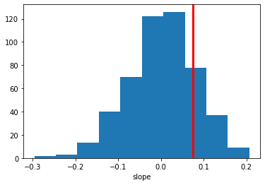
As you can see, the simulated data sets have on average no correlation to our trial-by-trial measure (just as in the data) but we also get a nice sense of the uncertainty in our estimation.