Network Inspectors
The network_inspectors() module allows you to inspect the LANs
directly. We will be grateful if you report any strange behavior you
might find.
# MODULE IMPORTS ----
import numpy as np
import hddm
Direct access to batch predictions
You can use the hddm.network_inspectors.get_torch_mlp() function to
access network predictions.
# Specify model
model = 'angle'
lan_angle = hddm.network_inspectors.get_torch_mlp(model = model)
# Make some random parameter set
parameter_df = hddm.simulators.make_parameter_vectors_nn(model = model,
                                                         param_dict = None,
                                                         n_parameter_vectors = 1)

parameter_matrix = np.tile(np.squeeze(parameter_df.values), (200, 1))

# Initialize network input
network_input = np.zeros((parameter_matrix.shape[0], parameter_matrix.shape[1] + 2)) # Note the + 2 on the right --> we append the parameter vectors with reaction times (+1 columns) and choices (+1 columns)

# Add reaction times
network_input[:, -2] = np.linspace(0, 3, parameter_matrix.shape[0])

# Add choices
network_input[:, -1] = np.repeat(np.random.choice([-1, 1]), parameter_matrix.shape[0])

# Note: The networks expects float32 inputs
network_input = network_input.astype(np.float32)

# Show example output
print('Some network outputs')
print(lan_angle(network_input)[:10]) # printing the first 10 outputs
print('Shape')
print(lan_angle(network_input).shape) # original shape of output
Some network outputs
[[-6.5302606 ]
 [ 0.5264375 ]
 [ 0.410895  ]
 [-0.52280986]
 [-1.0521754 ]
 [-1.552991  ]
 [-2.0735168 ]
 [-2.6183672 ]
 [-3.2071779 ]
 [-3.878473  ]]
Shape
(200, 1)
Plotting Utilities
HDDM provides two plotting function to investigate the network outputs
directly. The kde_vs_lan_likelihoods() plot and the
lan_manifold() plot.
NOTE: These utilities are designed for 2-choice models at the moment.
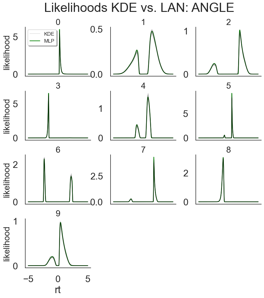
kde_vs_lan_likelihoods()
# Make some parameters
parameter_df = hddm.simulators.make_parameter_vectors_nn(model = model,
                                                         param_dict = None,
                                                         n_parameter_vectors = 10)
parameter_df
| v | a | z | t | theta | |
|---|---|---|---|---|---|
| 0 | 2.729321 | 1.184634 | 0.798893 | 0.186882 | 0.225510 |
| 1 | 0.550569 | 1.473085 | 0.389967 | 0.583149 | 0.317908 |
| 2 | 0.297733 | 1.241166 | 0.630780 | 1.617812 | 0.455768 |
| 3 | -2.918573 | 0.972126 | 0.307551 | 1.496773 | 0.898875 |
| 4 | 0.666445 | 1.882498 | 0.530820 | 0.259892 | 1.028040 |
| 5 | 1.629646 | 0.507156 | 0.692670 | 0.529111 | 0.845566 |
| 6 | -1.255036 | 1.741760 | 0.678846 | 1.849304 | 1.233386 |
| 7 | 0.891731 | 0.795798 | 0.721093 | 1.705487 | 0.704186 |
| 8 | -2.954760 | 1.518239 | 0.419388 | 0.623301 | 0.607989 |
| 9 | 0.360199 | 1.369782 | 0.629768 | 0.098295 | 0.497529 |
hddm.network_inspectors.kde_vs_lan_likelihoods(parameter_df = parameter_df,
                                               model = model,
                                               cols = 3,
                                               n_samples = 2000,
                                               n_reps = 10,
                                               show = True)
1 of 10
2 of 10
3 of 10
4 of 10
5 of 10
6 of 10
7 of 10
8 of 10
9 of 10
10 of 10
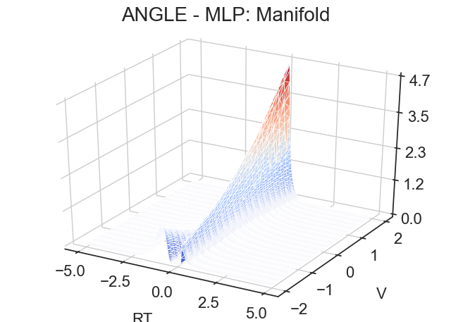
lan_manifold()
Lastly, you can use the lan_manifold() plot to investigate the LAN
likelihoods over a range of parameters.
The idea is to use a base parameter vector and vary one of the parameters in a prespecificed range.
This plot can be informative if you would like to understand better how a parameter affects model behavior.
# Now plotting
hddm.network_inspectors.lan_manifold(parameter_df = parameter_df,
                                     vary_dict = {'v': np.linspace(-2, 2, 20)},
                                     model = model,
                                     n_rt_steps = 300,
                                     fig_scale = 1.0,
                                     max_rt = 5,
                                     save = True,
                                     show = True)
Using only the first row of the supplied parameter array !