From simulator to Inference with HDDM (MNLE Version)

In this tutorial we show how to proceed from a simulator model to Bayesian Inference with HDDM, via training a likelihood approximator of the MNLE type.

MNLE stands for Mixed Neural Likelihood Estimator, which in turn is a Neural Network composed of the combination of a Flow, and a basic classifier MLP. MNLEs are designed for predicting (and generating data from) likelihoods over mixed data containing a continuous and a discrete part.

In the context of Sequential Sampling Models, the continuous part refers to the reaction times, while the discrete part refers to choices.

We will make use of two python packages which help facilitate this tutorial:

1. The `ssms <https://github.com/AlexanderFengler/ssm_simulators>`__ package, which holds a collection of fast simulators and training data generators for LANs (here we make use only of the basic simulators and ignore the LAN integration)

2. The `sbi <https://github.com/AlexanderFengler/LANfactory>`__ package, which makes training MNLEs easy. The package has a much broader scope, which we suggest the interested user to explore, however not all aspects of the sbi toolbox allow for an interface with HDDM.

In this tutorial we will start by simulating data from the DDM, using the `ssms <https://github.com/AlexanderFengler/ssm_simulators>`__, then use this data to train a MNLE via the `sbi <https://github.com/AlexanderFengler/LANfactory>`__ toolbox and finally define a wrapper around the resulting MNLE to make it usable in HDDM.

Installation (colab)

NOTE: If you run this Tutorial in a google colab, don’t forget to change the runtime to a GPU machine for better performance.

# !pip install sbi
# !pip install cython
# !pip install pymc==2.3.8
# !pip install git+https://github.com/hddm-devs/kabuki
# !pip install git+https://github.com/hddm-devs/hddm
# !pip install git+https://github.com/AlexanderFengler/ssm_simulators

Load Modules

# ssms for simulation
from ssms.basic_simulators import simulator

# sbi for network training
import sbi
from sbi.inference import MNLE

# HDDM
import hddm

# Misc
from copy import deepcopy
import ssms
import torch
import numpy as np
import pandas as pd
import matplotlib
import matplotlib.pyplot as plt

Simulate Data

from ssms.config import model_config

# Define our model
model = 'ddm'

# Load corresponding config dictionary
model_config_tmp = deepcopy(model_config['ddm'])
model_config_tmp["choices"] = [-1, 1] # simple addition to make ssms model config hddm ready

# Choose number of training examples
n_training_examples = 100000

# Generate a matrix of model parameters
# We sample this uniformly from an allowed parameter space
thetas = np.random.uniform(low = model_config_tmp['param_bounds'][0],
                           high = model_config_tmp['param_bounds'][1],
                           size = (n_training_examples, len(model_config_tmp['params'])))
thetas_torch = torch.Tensor(thetas)

# For every row in thetas, draw 1 sample from the DDM.
model_simulations = ssms.basic_simulators.simulator(model = 'ddm',
                                                    theta = thetas,
                                                    n_samples = 1)

# Format the output of the simulator
model_simulations_torch = torch.Tensor(np.hstack((model_simulations['rts'], model_simulations['choices'])))

# Edit choices to [0,1] (the simulator produces [-1, 1]) since that is the format MNLE expects.
model_simulations_torch[:, 1] = (model_simulations_torch[:, 1] + 1)/2

Train Network

# Set device
torch_device = torch.device("cuda") if torch.cuda.is_available() else torch.device("cpu")

#Initialise Prior
prior = sbi.utils.BoxUniform(low=torch.tensor(ssms.config.model_config['ddm']['param_bounds'][0]),
                             high=torch.tensor(ssms.config.model_config['ddm']['param_bounds'][1]),
                             device = torch_device.type)

# Initialise the MNLE trainer
trainer = MNLE(prior = prior,
               device = torch_device.type)

# Add presimulated training data to the MNLE trainer
trainer = trainer.append_simulations(thetas_torch,
                                     model_simulations_torch)

# Train the network and return the resulting MNLE
mnle = trainer.train(training_batch_size = 128 if torch_device.type == "cpu" else 1000)

/Users/afengler/opt/miniconda3/envs/hddmnn_tutorial/lib/python3.7/site-packages/sbi/neural_nets/mnle.py:64: UserWarning: The mixed neural likelihood estimator assumes that x contains
        continuous data in the first n-1 columns (e.g., reaction times) and
        categorical data in the last column (e.g., corresponding choices). If
        this is not the case for the passed x do not use this function.
  this is not the case for the passed x do not use this function."""

Neural network successfully converged after 74 epochs.

Run in HDDM

Define HDDM Network

class MNLEWrapper():
    def __init__(
        self, MNLE):
        self.mnle = MNLE
        self.dev = torch.device("cuda") if torch.cuda.is_available() else torch.device("cpu")

    # We need to define a predict on batch method for compatibility with HDDM
    def predict_on_batch(self, data):
        # HDDM supplies decisions as [-1, 1], which we adjust
        # to [0, 1] for the MNLE
        data[:, -1] = (data[:, -1] + 1) / 2

        return self.mnle.log_prob(torch.tensor(data[:,-2:]).to(self.dev), # supply (rt, choice)
                                  torch.tensor(data[:,:-2]).to(self.dev) # supply (theta)
                                  ).cpu().detach().numpy() # send back to cpu (for MCMC sampler to proceed)

The argument x, to the predict_on_batch(), when called from within HDDM’s sampler, will be a matrix. Rows correspond to trials, and columns are supplied in the following way.

The first few columns contain trial wise parameters (in the order specific in the model_config above under the "params" key). The last two columns contain the trial wise reaction times and choices respectively.

To understand how the network is actually called in HDDM, let’s take a peak into the generic internal likelihood function.

NOTE: Don’t actually run the cell below. It is just for illustration.

def wiener_like_nn_mlp_pdf(np.ndarray[float, ndim = 1] rt,
                           np.ndarray[float, ndim = 1] response,
                           np.ndarray[float, ndim = 1] params,
                           double p_outlier = 0,
                           double w_outlier = 0,
                           bint logp = 0,
                           network = None):

    cdef Py_ssize_t size = rt.shape[0]
    cdef Py_ssize_t n_params = params.shape[0]

    cdef np.ndarray[float, ndim = 1] log_p = np.zeros(size, dtype = np.float32)
    cdef float ll_min = -16.11809

    cdef np.ndarray[float, ndim = 2] data = np.zeros((size, n_params + 2), dtype = np.float32)
    data[:, :n_params] = np.tile(params, (size, 1)).astype(np.float32)
    data[:, n_params:] = np.stack([rt, response], axis = 1)

    # Call to network:
    if p_outlier == 0:
        log_p = np.squeeze(np.core.umath.maximum(network.predict_on_batch(data), ll_min))
    else: # ddm_model
        log_p = np.squeeze(np.log(np.exp(np.core.umath.maximum(network.predict_on_batch(data), ll_min)) * (1.0 - p_outlier) + (w_outlier * p_outlier)))
    if logp == 0:
        log_p = np.exp(log_p)
    return log_p

We see that the internal likelihood function expects a network as input and then finally calls the predict_on_batch() to get log-likelihoods.

We can now initialize the HDDM-ready MNLE via our MNLEWrapper() class, after which we are essentially good to go for an HDDM application.

# Initalize HDDM ready MNLE
mnle_hddm = MNLEWrapper(MNLE = mnle)

Generate Example Data

# Choose some parameters
v = 0.9
a = 1.4
z = 0.45
t = 0.7

# Simulate Data
data = ssms.basic_simulators.simulator(model = model,
                                       theta = [v, a, z, t],
                                       n_samples = 500)

# Bring into correct shape expected from HDDM
data_df = pd.DataFrame(np.stack([data['rts'], data['choices']], axis = 1)[:, :, 0],
                       columns = ['rt', 'response'])
data_df['subj_idx'] = 0
data_df['v'] = v
data_df['a'] = a
data_df['z'] = z
data_df['t'] = t

data_df

	rt	response	subj_idx	v	a	z	t
0	1.106998	1.0	0	0.9	1.4	0.45	0.7
1	1.396995	1.0	0	0.9	1.4	0.45	0.7
2	2.062008	1.0	0	0.9	1.4	0.45	0.7
3	5.708819	1.0	0	0.9	1.4	0.45	0.7
4	1.877999	1.0	0	0.9	1.4	0.45	0.7
...	...	...	...	...	...	...	...
495	3.119007	1.0	0	0.9	1.4	0.45	0.7
496	1.972003	1.0	0	0.9	1.4	0.45	0.7
497	1.719992	1.0	0	0.9	1.4	0.45	0.7
498	1.735992	1.0	0	0.9	1.4	0.45	0.7
499	2.010005	1.0	0	0.9	1.4	0.45	0.7

500 rows × 7 columns

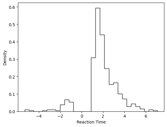
# Plotting the RTs
plt.hist(data_df['rt'] * data_df['response'],
         histtype = 'step',
         color = 'black',
         density = True,
         bins = 30)
plt.xlabel('Reaction Time')
plt.ylabel('Density')
plt.show()

Define HDDM Model

# Define the HDDM model
hddmmnle_model = hddm.HDDMnn(data = data_df,
                             informative = False,
                             include = model_config_tmp['hddm_include'],# Note: This include statement is an example, you may pick any other subset of the parameters of your model here
                             model = model,
                             model_config = model_config_tmp,
                             network = mnle_hddm)

Supplied model_config does not have a params_std_upper argument.
Set to a default of 10
Supplied model_config does not have a params_std_upper argument.
Set to a default of 10
Supplied model_config does not have a params_std_upper argument.
Set to a default of 10
Supplied model_config does not have a params_std_upper argument.
Set to a default of 10

Sample

# Sample from the model
n_mcmc = 1000
n_burn = 100

hddmmnle_model.sample(n_mcmc, burn = n_burn)

[-----------------100%-----------------] 1001 of 1000 complete in 360.0 sec

<pymc.MCMC.MCMC at 0x16d777490>

# Show posterior summary
tmp = hddmmnle_model.gen_stats()
tmp['ground_truth'] = data_df.iloc[0, 3:]
tmp[['ground_truth', 'mean', 'std']]

	ground_truth	mean	std
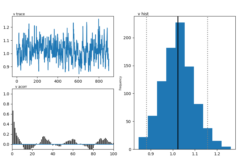
v	0.90	1.024209	0.071095
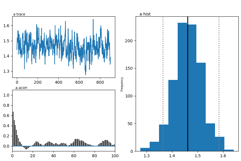
a	1.40	1.461075	0.054512
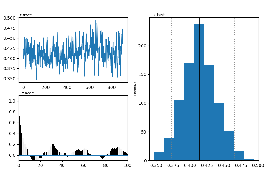
z	0.45	0.413947	0.02392
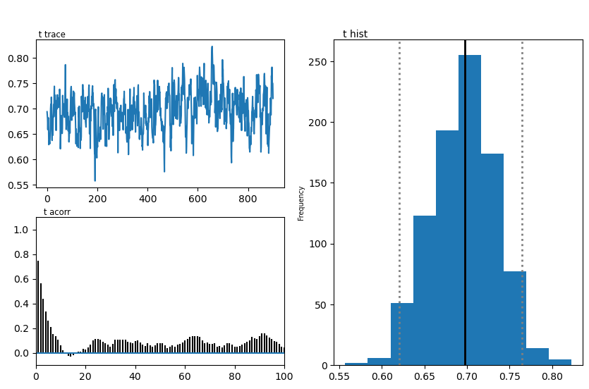
t	0.70	0.695977	0.037936

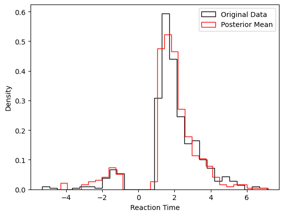
Plots

We show two plots. First, we compare simulations fixing the parameters at the posterior mean with the original data, to get a visual idea of the model fit we obtained. Second we show the posterior traces.

# Compare simulations from posterior mean parameters
# to original data
data_post_mean = data = ssms.basic_simulators.simulator(model = model,
                                                        theta = list(tmp['mean'].values),
                                                        n_samples = 500)


# Plotting the RTs
plt.hist(data_df['rt'] * data_df['response'],
         histtype = 'step',
         color = 'black',
         density = True,
         bins = 30,
         label = 'Original Data')
plt.hist(data_post_mean['rts'] * data_post_mean['choices'],
         histtype = 'step',
         color = 'red',
         density = True,
         bins = 30,
         label = 'Posterior Mean')
plt.xlabel('Reaction Time')
plt.ylabel('Density')
plt.legend()
plt.show()

# Plot the posteriors
hddmmnle_model.plot_posteriors()
plt.show()

Plotting v
Plotting a
Plotting z
Plotting t