New Visualizations
import hddm
from matplotlib import pyplot as plt
import numpy as np
from copy import deepcopy
Generate some Data
# Metadata
nmcmc = 2000
model = 'angle'
n_samples = 1000
includes = hddm.simulators.model_config[model]['hddm_include']
data, full_parameter_dict = hddm.simulators.hddm_dataset_generators.simulator_h_c(n_subjects = 5,
                                                                                  n_trials_per_subject = n_samples,
                                                                                  model = model,
                                                                                  p_outlier = 0.00,
                                                                                  conditions = None,
                                                                                  depends_on = None,
                                                                                  regression_models = None,
                                                                                  regression_covariates = None,
                                                                                  group_only_regressors = False,
                                                                                  group_only = None,
                                                                                  fixed_at_default = None)
data
| rt | response | subj_idx | v | a | z | t | theta | |
|---|---|---|---|---|---|---|---|---|
| 0 | 1.590851 | 0.0 | 0 | -1.704336 | 0.917225 | 0.612362 | 0.898857 | 0.251476 |
| 1 | 1.784849 | 0.0 | 0 | -1.704336 | 0.917225 | 0.612362 | 0.898857 | 0.251476 |
| 2 | 1.927849 | 0.0 | 0 | -1.704336 | 0.917225 | 0.612362 | 0.898857 | 0.251476 |
| 3 | 1.390854 | 0.0 | 0 | -1.704336 | 0.917225 | 0.612362 | 0.898857 | 0.251476 |
| 4 | 1.839848 | 0.0 | 0 | -1.704336 | 0.917225 | 0.612362 | 0.898857 | 0.251476 |
| ... | ... | ... | ... | ... | ... | ... | ... | ... |
| 4995 | 1.441180 | 0.0 | 4 | -1.314454 | 1.491856 | 0.488526 | 0.915183 | 0.119143 |
| 4996 | 1.239182 | 0.0 | 4 | -1.314454 | 1.491856 | 0.488526 | 0.915183 | 0.119143 |
| 4997 | 1.708176 | 0.0 | 4 | -1.314454 | 1.491856 | 0.488526 | 0.915183 | 0.119143 |
| 4998 | 1.447180 | 0.0 | 4 | -1.314454 | 1.491856 | 0.488526 | 0.915183 | 0.119143 |
| 4999 | 1.729176 | 0.0 | 4 | -1.314454 | 1.491856 | 0.488526 | 0.915183 | 0.119143 |
5000 rows × 8 columns
# Define the HDDM model
hddmnn_model = hddm.HDDMnn(data,
                           informative = False,
                           include = includes,
                           p_outlier = 0.0,
                           model = model)
# Sample
hddmnn_model.sample(nmcmc,
                    burn = 100)
[-----------------100%-----------------] 2000 of 2000 complete in 450.8 sec
<pymc.MCMC.MCMC at 0x14342cdd0>
hddm.plotting.plot_posterior_predictive(model = hddmnn_model,
                                        columns = 2, # groupby = ['subj_idx'],
                                        figsize = (12, 8),
                                        value_range = np.arange(0, 3, 0.1),
                                        plot_func = hddm.plotting._plot_func_model,
                                        parameter_recovery_mode = True,
                                        **{'add_legend': False,
                                           'alpha': 0.01,
                                           'ylim': 6.0,
                                           'bin_size': 0.025,
                                           'add_posterior_mean_model': True,
                                           'add_posterior_mean_rts': True,
                                           'add_posterior_uncertainty_model': True,
                                           'add_posterior_uncertainty_rts': False,
                                           'samples': 200,
                                           'legend_fontsize': 7,
                                           'legend_loc': 'upper left',
                                           'linewidth_histogram': 1.0,
                                           'subplots_adjust': {'top': 0.9, 'hspace': 0.35, 'wspace': 0.3}})
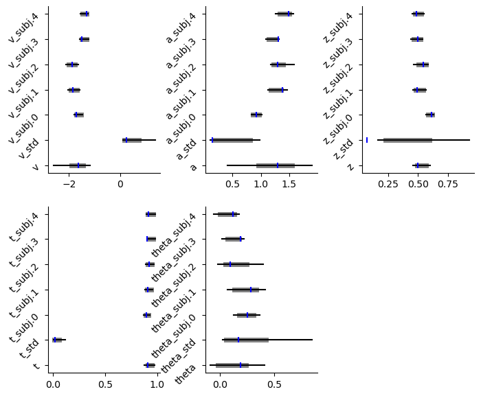
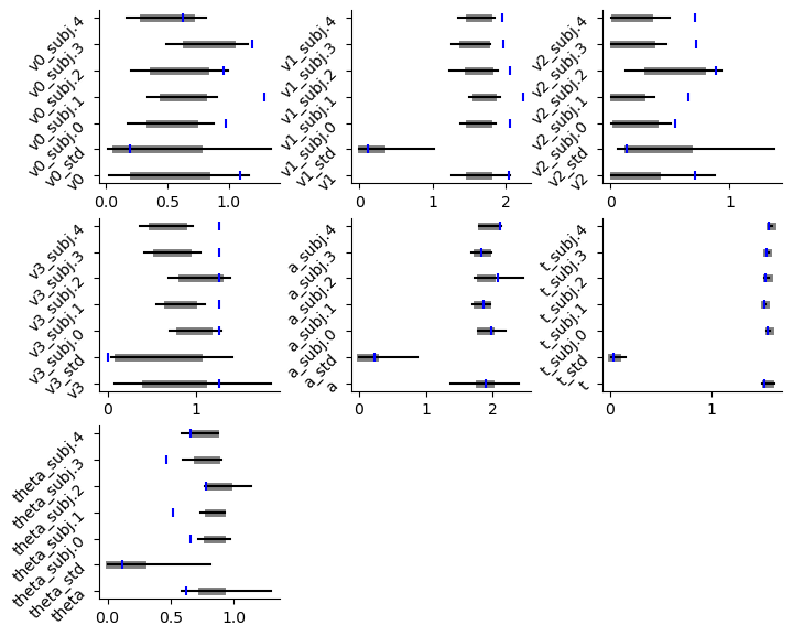
caterpillar plot
The caterpillar_plot() function below displays parameterwise,
as a blue tick-mark the ground truth.
as a thin black line the \(1 - 99\) percentile range of the posterior distribution
as a thick black line the \(5-95\) percentile range of the posterior distribution
Again use the help() function to learn more.
# Caterpillar Plot: (Parameters recovered ok?)
hddm.plotting.plot_caterpillar(hddm_model = hddmnn_model,
                               ground_truth_parameter_dict = full_parameter_dict,
                               drop_sd = False,
                               figsize = (8, 6))
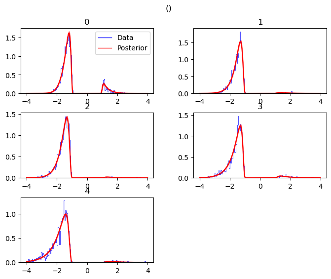
posterior predictive (standard)
We have two versions of the standard posterior predictive plots. Both
are called via the plot_posterior_predictive function, however you
pick the plot_func argument accordingly.
If you pick hddm.plotting.plot_func_posterior_pdf_node_nn, the
resulting plot uses likelihood pdf evaluations to show you the
posterior predictive including uncertainty.
If you pick hddm.plotting.plot_func_posterior_pdf_node_from_sim, the
posterior predictives instead derive from actual simulation runs from
the model.
Both function have a number of options to customize styling.
Below we illustrate:
_plot_func_posterior_pdf_node_nn
hddm.plotting.plot_posterior_predictive(model = hddmnn_model,
                                        columns = 2, # groupby = ['subj_idx'],
                                        figsize = (8, 6),
                                        value_range = np.arange(-4, 4, 0.01),
                                        plot_func = hddm.plotting._plot_func_posterior_pdf_node_nn,
                                        parameter_recovery_mode = True,
                                        **{'alpha': 0.01,
                                           'ylim': 3,
                                           'bin_size': 0.05,
                                           'add_posterior_mean_rts': True,
                                           'add_posterior_uncertainty_rts': True,
                                           'samples': 200,
                                           'legend_fontsize': 7,
                                           'subplots_adjust': {'top': 0.9, 'hspace': 0.3, 'wspace': 0.3}})
plt.show()
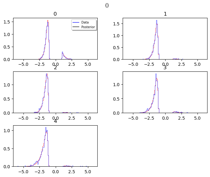
_plot_func_posterior_node_from_sim
hddm.plotting.plot_posterior_predictive(model = hddmnn_model,
                                        columns = 2, # groupby = ['subj_idx'],
                                        figsize = (8, 6),
                                        value_range = np.arange(-6, 6, 0.02),
                                        plot_func = hddm.plotting._plot_func_posterior_node_from_sim,
                                        parameter_recovery_mode = True,
                                        **{'alpha': 0.01,
                                           'ylim': 3,
                                           'bin_size': 0.1,
                                           'add_posterior_mean_rts': True,
                                           'add_posterior_uncertainty_rts': False,
                                           'samples': 200,
                                           'legend_fontsize': 7,
                                           'subplots_adjust': {'top': 0.9, 'hspace': 0.3, 'wspace': 0.3}})
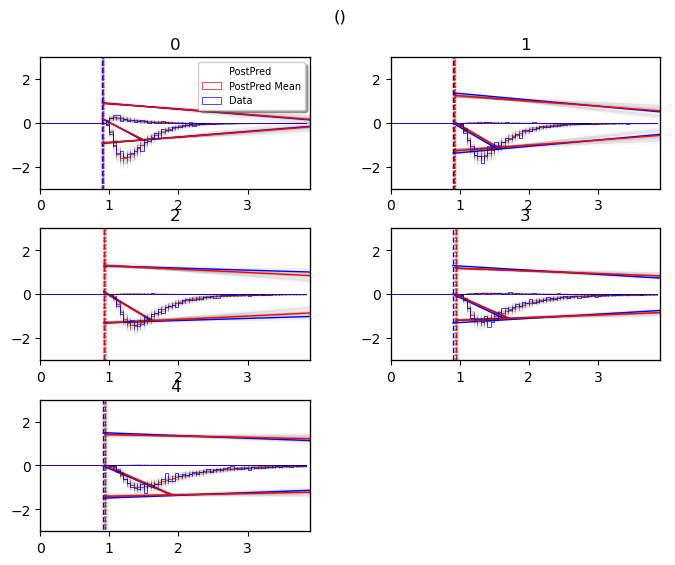
posterior predictive (model cartoon)
The model plot is useful to illustrate the behavior of a models pictorially, including the uncertainty over model parameters embedded in the posterior distribution.
This plot works only for 2-choice models at this point.
Check out more of it’s capabilities with the help() function.
hddm.plotting.plot_posterior_predictive(model = hddmnn_model,
                                        columns = 2, # groupby = ['subj_idx'],
                                        figsize = (8, 6),
                                        value_range = np.arange(0, 4, 0.1),
                                        plot_func = hddm.plotting._plot_func_model,
                                        parameter_recovery_mode = True,
                                        **{'alpha': 0.01,
                                           'ylim': 3,
                                           'add_posterior_mean_model': True,
                                           'add_posterior_mean_rts': True,
                                           'add_posterior_uncertainty_model': True,
                                           'add_posterior_uncertainty_rts': True,
                                           'samples': 200,
                                           'legend_fontsize': 7,
                                           'subplots_adjust': {'top': 0.9, 'hspace': 0.3, 'wspace': 0.3}})
plt.show()
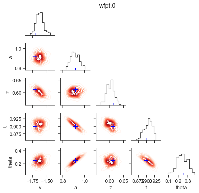
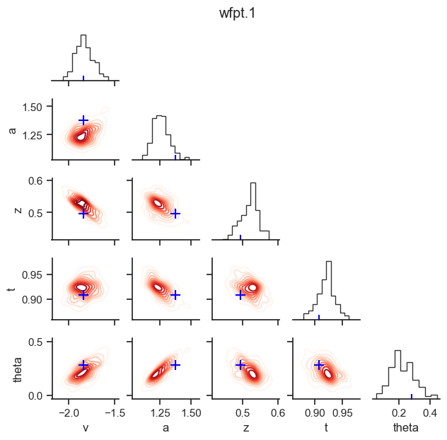
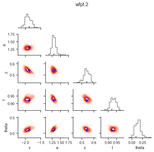
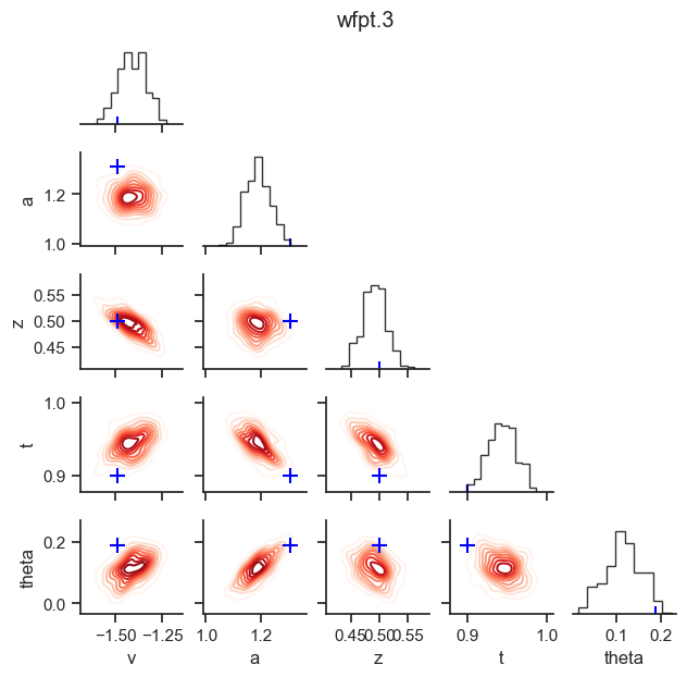
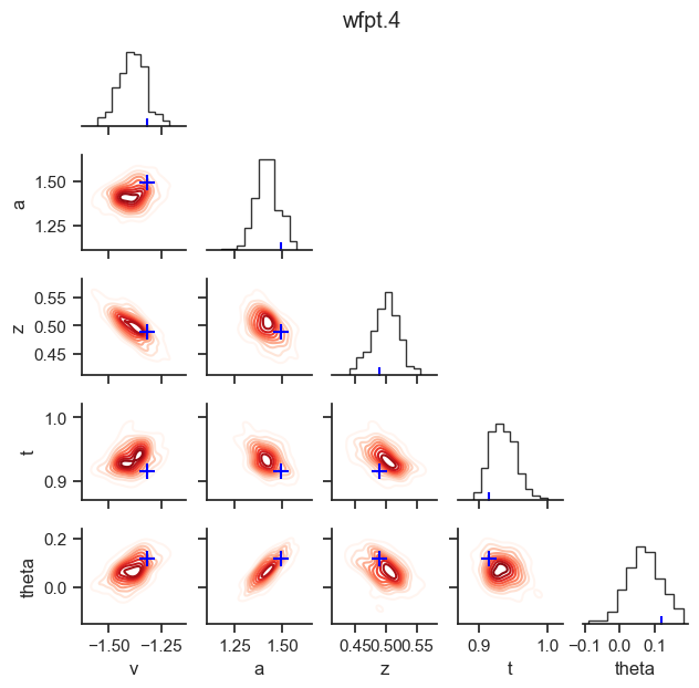
posterior pair plot
hddm.plotting.plot_posterior_pair(hddmnn_model, save = False,
                                  parameter_recovery_mode = True,
                                  samples = 200,
                                  figsize = (6, 6))
NEW (v0.9.3): Plots for \(n>2\) choice models
# Metadata
nmcmc = 1000
model = 'race_no_bias_angle_4'
n_samples = 1000
includes = deepcopy(hddm.simulators.model_config[model]['hddm_include'])
includes.remove('z')
data, full_parameter_dict = hddm.simulators.hddm_dataset_generators.simulator_h_c(n_subjects = 5,
                                                                                  n_trials_per_subject = n_samples,
                                                                                  model = model,
                                                                                  p_outlier = 0.00,
                                                                                  conditions = None,
                                                                                  depends_on = None,
                                                                                  regression_models = None,
                                                                                  regression_covariates = None,
                                                                                  group_only_regressors = False,
                                                                                  group_only = None,
                                                                                  fixed_at_default = ['z'])
data
| rt | response | subj_idx | v0 | v1 | v2 | v3 | a | z | t | theta | |
|---|---|---|---|---|---|---|---|---|---|---|---|
| 0 | 1.723548 | 1.0 | 0 | 0.973732 | 2.066200 | 0.541262 | 1.266078 | 1.988639 | 0.5 | 1.559548 | 0.656266 |
| 1 | 1.784549 | 2.0 | 0 | 0.973732 | 2.066200 | 0.541262 | 1.266078 | 1.988639 | 0.5 | 1.559548 | 0.656266 |
| 2 | 2.076545 | 3.0 | 0 | 0.973732 | 2.066200 | 0.541262 | 1.266078 | 1.988639 | 0.5 | 1.559548 | 0.656266 |
| 3 | 1.811549 | 3.0 | 0 | 0.973732 | 2.066200 | 0.541262 | 1.266078 | 1.988639 | 0.5 | 1.559548 | 0.656266 |
| 4 | 1.748549 | 3.0 | 0 | 0.973732 | 2.066200 | 0.541262 | 1.266078 | 1.988639 | 0.5 | 1.559548 | 0.656266 |
| ... | ... | ... | ... | ... | ... | ... | ... | ... | ... | ... | ... |
| 4995 | 1.931315 | 1.0 | 4 | 0.622314 | 1.956002 | 0.706355 | 1.264215 | 2.106691 | 0.5 | 1.569316 | 0.661371 |
| 4996 | 1.851316 | 1.0 | 4 | 0.622314 | 1.956002 | 0.706355 | 1.264215 | 2.106691 | 0.5 | 1.569316 | 0.661371 |
| 4997 | 1.910315 | 3.0 | 4 | 0.622314 | 1.956002 | 0.706355 | 1.264215 | 2.106691 | 0.5 | 1.569316 | 0.661371 |
| 4998 | 1.751316 | 1.0 | 4 | 0.622314 | 1.956002 | 0.706355 | 1.264215 | 2.106691 | 0.5 | 1.569316 | 0.661371 |
| 4999 | 1.908315 | 0.0 | 4 | 0.622314 | 1.956002 | 0.706355 | 1.264215 | 2.106691 | 0.5 | 1.569316 | 0.661371 |
5000 rows × 11 columns
# Define the HDDM model
hddmnn_model = hddm.HDDMnn(data,
                           informative = False,
                           include = includes,
                           p_outlier = 0.0,
                           model = model)
# Sample
hddmnn_model.sample(nmcmc,
                    burn = 100)
[-----------------100%-----------------] 1001 of 1000 complete in 475.6 sec
<pymc.MCMC.MCMC at 0x106755050>
caterpillar plot
# Caterpillar Plot: (Parameters recovered ok?)
hddm.plotting.plot_caterpillar(hddm_model = hddmnn_model,
                               ground_truth_parameter_dict = full_parameter_dict,
                               drop_sd = False,
                               figsize = (8, 6))
plt.show()
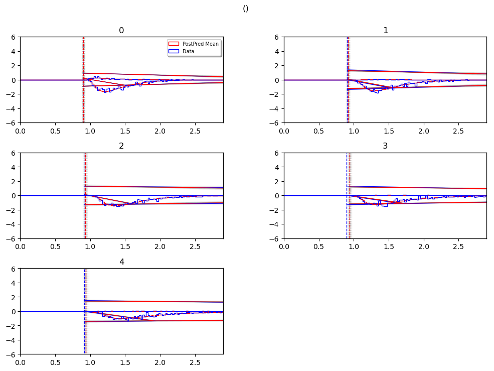
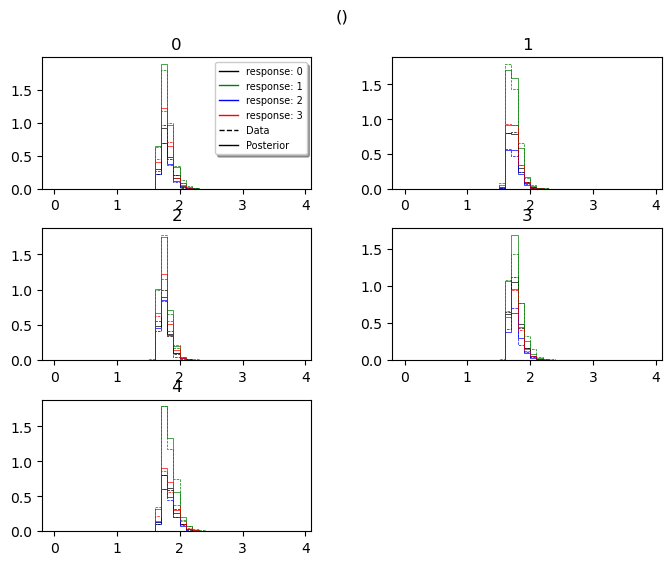
posterior_predictive_plot
hddm.plotting.plot_posterior_predictive(model = hddmnn_model,
                                        columns = 2, # groupby = ['subj_idx'],
                                        figsize = (8, 6),
                                        value_range = np.arange(0, 4, 0.02),
                                        plot_func = hddm.plotting._plot_func_posterior_node_from_sim,
                                        parameter_recovery_mode = True,
                                        **{'alpha': 0.01,
                                           'ylim': 3,
                                           'bin_size': 0.1,
                                           'add_posterior_mean_rts': True,
                                           'add_posterior_uncertainty_rts': False,
                                           'samples': 200,
                                           'legend_fontsize': 7,
                                           'subplots_adjust': {'top': 0.9, 'hspace': 0.3, 'wspace': 0.3}})
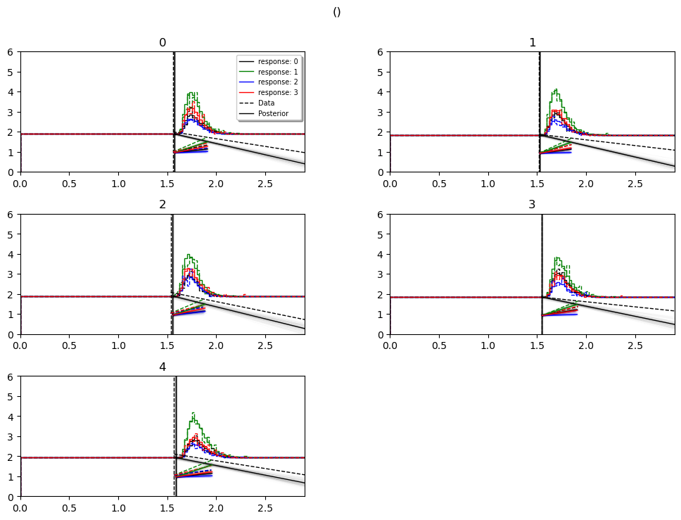
model_cartoon_plot
WARNING: The plot below should not be taken as representative for a particular model fit. The chain may need to be run for much longer than the number of samples allotted in this tutorial script.
hddm.plotting.plot_posterior_predictive(model = hddmnn_model,
                                        columns = 2, # groupby = ['subj_idx'],
                                        figsize = (12, 8),
                                        value_range = np.arange(0, 3, 0.1),
                                        plot_func = hddm.plotting._plot_func_model_n,
                                        parameter_recovery_mode = True,
                                        **{'add_legend': False,
                                           'alpha': 0.01,
                                           'ylim': 6.0,
                                           'bin_size': 0.025,
                                           'add_posterior_mean_model': True,
                                           'add_posterior_mean_rts': True,
                                           'add_posterior_uncertainty_model': True,
                                           'add_posterior_uncertainty_rts': False,
                                           'samples': 200,
                                           'legend_fontsize': 7,
                                           'legend_loc': 'upper left',
                                           'linewidth_histogram': 1.0,
                                           'subplots_adjust': {'top': 0.9, 'hspace': 0.35, 'wspace': 0.3}})
plt.show()